Tensor or field surrogates
Contents
Tensor or field surrogates#
In order to fit tensors or fields, i.e., a multi-output or multi-target machine learning regression, we can utilize the multiple PCE regression wrapper which is part of tesuract’s toolbox.
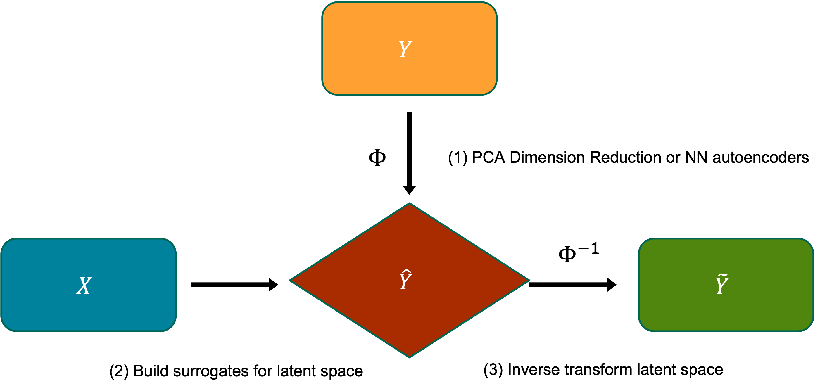
In a nutshell, tesuract uses sklearn’s Pipeline machinery to (1) transform the target into a lower-dimensional latent space, typically through PCA, (2) then creates a separately tuned surrogate for each of the latent space dimensions, and then (3) projects the solution back into the physical space.
This is summarized in the image below.
tesuract_pipeline.png#
Let’s see how to perform this fit using the tools in tesuract. First, we will need to import a relevant data set which we have conveniently added to the data folder in the tests directory.
import numpy as np
import tesuract
%matplotlib inline

# load the relevant data set
loaddir = "../../../tesuract/tests/data/"
X = np.loadtxt("rom_test_X.txt")
Y = np.loadtxt("rom_test_Y.txt")

# print out the shapes of the input and output
X.shape, Y.shape
((100, 2), (100, 288))
As one can see, the input is a two-dimensional feature space, but the output is a 288-dimensional field or tensor.
Now, we can fit each and every one of the 288 outputs with a ML regressor, but if we were to utilize hyper-parameter tuning (and we should if we can), this would be extremely expensive and cumbersome.
Instead, we introduce a target transform which takes the output and projects it onto a lower-dimensional latent space, after which, we do all our fitting.
PCA target transform#
Let’s define a simple target transform using sklearn’s PCA with say 4 components. In general, we can make the choice of this automatic, but for now, let’s define the number of components or latent space dimensions. All we need to do is call sklearn’s PCA and feed it in some parameter options as a dictionary.
from sklearn.decomposition import PCA
Now, all we do is call tesuract.MRegressionWrapperCV which is almost
identical to tesuract.RegressionWrapperCV except that we can feed it
in a target transform (Note that any sklearn transform will work here,
even a simple scalar transform, although that doesn’t save you in terms
of computational cost).
# define pce grid again
pce_grid = {
    'order': list(range(1,8)),
    'mindex_type': ['total_order'],
    'fit_type': ['ElasticNetCV'],
    }

mpce = tesuract.MRegressionWrapperCV(
    regressor='pce',
    reg_params=pce_grid,
    target_transform=PCA,
    target_transform_params={'n_components':4})
And that’s it! Now we can feed it in our multi-target training data pair (X,Y). This will take a little bit of time since we are fitting each of the 8 components with a PCE. While this is done in serial, each hyper-parameter search is done in parallel.
mpce.fit(X,Y)
on 0: Fitting 5 folds for each of 7 candidates, totalling 35 fits
on 1: Fitting 5 folds for each of 7 candidates, totalling 35 fits
on 2: Fitting 5 folds for each of 7 candidates, totalling 35 fits
on 3: Fitting 5 folds for each of 7 candidates, totalling 35 fits
|████████████████████████████████████████| 4/4 [100%] in 5.8s (0.70/s)
MRegressionWrapperCV(cv=KFold(n_splits=5, random_state=None, shuffle=False),
                     reg_params={'fit_type': ['ElasticNetCV'],
                                 'mindex_type': ['total_order'],
                                 'order': [1, 2, 3, 4, 5, 6, 7]},
                     target_transform=<class 'sklearn.decomposition._pca.PCA'>,
                     target_transform_params={'n_components': 4})
Once this is complete, we can view the best estimators for each of the components, along with their respective scores and parameters.
# show the parameters of the best fit PCEs for the four components
mpce.best_params_
[{'fit_type': 'ElasticNetCV', 'mindex_type': 'total_order', 'order': 6},
 {'fit_type': 'ElasticNetCV', 'mindex_type': 'total_order', 'order': 5},
 {'fit_type': 'ElasticNetCV', 'mindex_type': 'total_order', 'order': 1},
 {'fit_type': 'ElasticNetCV', 'mindex_type': 'total_order', 'order': 3}]
# extract the best estimators for each component
best_estimators = mpce.best_estimators_
# we can also output the best scores, which by default is the
#   negative root mean squared error
# Note that this can be set to any number of the regression scores
#   used in sklearn's metric library.
mpce.best_scores_
[-49.341166974922444,
 -23.822169033173523,
 -24.2500961913357,
 -14.222838497441805]
To make predictions using the best estimators, one can simply use the predict method, which is automatically use the best estimators to make the prediction.
mpce.predict(X)
array([[-5.9192281 , -6.29485307, -6.29485307, ...,  0.        ,
         0.        ,  0.        ],
       [-5.84729987, -6.19757176, -6.19757176, ...,  0.        ,
         0.        ,  0.        ],
       [-5.95122359, -6.34418361, -6.34418361, ...,  0.        ,
         0.        ,  0.        ],
       ...,
       [-5.89743814, -6.26569268, -6.26569268, ...,  0.        ,
         0.        ,  0.        ],
       [-5.80345682, -6.13921674, -6.13921674, ...,  0.        ,
         0.        ,  0.        ],
       [-5.94735135, -6.39569148, -6.39569148, ...,  0.        ,
         0.        ,  0.        ]])
Note that one can define a whole slew of options in the PCE parameter grid. For example, when using LassoCV, it might be necessary to increase the maximum iteration or the tolerance. In this case, one can easily modify the grid to look like the following.
Scoring tensor surrogate estimators#
Once we obtain a set of best estimators for each component, we have our full tensor surrogate model. Moreover, we have a sense of how good it is by looking at the cross-validation scores for each latent space fitting. However, a more accurate score would be to look at the cross-validation values for the full model in the physical space (not the latent space).
The simplest way to compute this would be to pass the mpce object to
the cross_val_score method in sklearn’s toolbox. The draw back here
is that for each train/ test split, it will perform a completely new
hyper-parameter grid search over the original parameter grid. This can
be computationally burdensome. Instead, we can create a surrogate clone
using the selected set of best parameters from the calculations above.
In the future, we should make this clone easily extractable from the tool box, but for now, we can manually create a cloned surrogate with predefined parameter grids corresponding to the optimal findings.
# Set the number of component to model value
n_components = 4

# We will feed MRregressionWrapperCV a list of regressors
#     and parameter grid specifying the exact values
reg_custom_list = ['pce' for i in range(n_components)]
reg_param_list = mpce.best_params_ # important step to speed up cv score

# now we create a clone of the surrogate setting custom_params=True
clone = tesuract.MRegressionWrapperCV(
    regressor=reg_custom_list,
    reg_params=reg_param_list,
    custom_params = True,
    target_transform=PCA(n_components=4),
    target_transform_params={},
    n_jobs=-1,verbose=0)
Now, we can feed the clone function into sklearn’s cross validation score.
from sklearn.model_selection import cross_val_score
mpce_score = cross_val_score(clone,X,Y)
print("PCE score is {0:.3f}".format(mpce_score.mean()))
|████████████████████████████████████████| 4/4 [100%] in 0.7s (5.46/s)
|████████████████████████████████████████| 4/4 [100%] in 0.7s (5.59/s)
|████████████████████████████████████████| 4/4 [100%] in 0.7s (5.92/s)
|████████████████████████████████████████| 4/4 [100%] in 0.8s (5.06/s)
on 0: /Users/kchowdh/.pyenv/versions/3.8.10/lib/python3.8/site-packages/sklearn/linear_model/_coordinate_descent.py:633: ConvergenceWarning: Objective did not converge. You might want to increase the number of iterations. Duality gap: 2310.710683199475, tolerance: 1805.4727026258927
        model = cd_fast.enet_coordinate_descent_gram(
|████████████████████████████████████████| 4/4 [100%] in 0.7s (5.52/s)
PCE score is -0.007
# default score is a negative relative error but can be modified with any
#    custom scorer
mpce_score
array([-0.00857342, -0.00740425, -0.00610879, -0.00652324, -0.00651267])
Custom scorer for field functions#
Here is a simple example of a custom relative error scorer for field functions. One can also use something as simple as an R-squared score, which compute the traditional scalar R-squared score for each target and then averages them together.
# example custom scorer
from sklearn.metrics import make_scorer
def my_scorer(ytrue,ypred):
    # (negative) relative mean square error score
    mse = np.mean((ytrue - ypred)**2)/np.mean(ytrue**2)
    return -mse
custom_scorer = make_scorer(my_scorer, greater_is_better=True)
More advanced hyper-parameter tuning#
In some cases, it may be useful to more explicity with the parameter grid. In this case, we will define a different parameter grid for LassoCV than for ElasticNet. Moreover, we will utilize a different constructor for the parameter grid where we input a list instead of a string. The neat thing with this approach is that we can feed our resuract regressor a bunch of different machine learning regressors and it will return the best among them. Moreso, for the multi-target tensor fits, it can possibly return a mixed model where some component may be a different type of ML model!
# PCE grid with different parameters for ElasticNetCV vs LassoCV
pce_grid = [
    {'order': list(range(1,10)),
    'mindex_type': ['total_order','hyperbolic'],
    'fit_type': ['linear','ElasticNetCV'],
    'fit_params': [{'alphas':np.logspace(-8,4,20),'max_iter':100000,'tol':5e-2}]
    },
    {'order': list(range(1,10)),
    'mindex_type': ['total_order','hyperbolic'],
    'fit_type': ['LassoCV'],
    'fit_params': [{'alphas':np.logspace(-8,3,15),'max_iter':500000,'tol':1.5e-1}]}
     ]

# Construct a surrogate by feeding in a list of regressors and grids
mpce2 = tesuract.MRegressionWrapperCV(
    regressor=['pce'],
    reg_params=[pce_grid],
    target_transform=PCA,
    target_transform_params={'n_components':4})

# mpce2.fit(X,Y)
mpce.best_params_
[{'fit_type': 'ElasticNetCV', 'mindex_type': 'total_order', 'order': 6},
 {'fit_type': 'ElasticNetCV', 'mindex_type': 'total_order', 'order': 5},
 {'fit_type': 'ElasticNetCV', 'mindex_type': 'total_order', 'order': 1},
 {'fit_type': 'ElasticNetCV', 'mindex_type': 'total_order', 'order': 3}]
Mixed regression models#
Let’s take the above and also compare to random forests!
from sklearn.ensemble import RandomForestRegressor

pce_grid = [
    {'order': list(range(1,10)),
    'mindex_type': ['total_order','hyperbolic'],
    'fit_type': ['linear','ElasticNetCV'],
    'fit_params': [{'alphas':np.logspace(-8,4,20),'max_iter':100000,'tol':5e-2}]
    }]

rf_grid = {
    'n_estimators': [200,500],
    'max_depth': [3,5,10]
    }

# Construct a surrogate by feeding in a list of regressors and grids
mpce_mixed = tesuract.MRegressionWrapperCV(
    regressor=['pce','rf'],
    reg_params=[pce_grid,rf_grid],
    target_transform=PCA,
    target_transform_params={'n_components':4})

mpce_mixed.fit(X,Y)
on 0: Fitting 5 folds for each of 36 candidates, totalling 180 fits
on 0: Fitting 5 folds for each of 6 candidates, totalling 30 fits
on 1: Fitting 5 folds for each of 36 candidates, totalling 180 fits
on 1: Fitting 5 folds for each of 6 candidates, totalling 30 fits
on 2: Fitting 5 folds for each of 36 candidates, totalling 180 fits
on 2: Fitting 5 folds for each of 6 candidates, totalling 30 fits
on 3: Fitting 5 folds for each of 36 candidates, totalling 180 fits
on 3: Fitting 5 folds for each of 6 candidates, totalling 30 fits
|████████████████████████████████████████| 4/4 [100%] in 1:07.5 (0.06/s)
MRegressionWrapperCV(cv=KFold(n_splits=5, random_state=None, shuffle=False),
                     reg_params=[[{'fit_params': [{'alphas': array([1.00000000e-08, 4.28133240e-08, 1.83298071e-07, 7.84759970e-07,
       3.35981829e-06, 1.43844989e-05, 6.15848211e-05, 2.63665090e-04,
       1.12883789e-03, 4.83293024e-03, 2.06913808e-02, 8.85866790e-02,
       3.79269019e-01, 1.62377674e+00, 6.95192796e+00, 2.9763...
       1.27427499e+02, 5.45559478e+02, 2.33572147e+03, 1.00000000e+04]),
                                                   'max_iter': 100000,
                                                   'tol': 0.05}],
                                   'fit_type': ['linear', 'ElasticNetCV'],
                                   'mindex_type': ['total_order', 'hyperbolic'],
                                   'order': [1, 2, 3, 4, 5, 6, 7, 8, 9]}],
                                 {'max_depth': [3, 5, 10],
                                  'n_estimators': [200, 500]}],
                     regressor=['pce', 'rf'],
                     target_transform=<class 'sklearn.decomposition._pca.PCA'>,
                     target_transform_params={'n_components': 4})
# Let's show which type of estimators came out best: RF vs PCE
[t['fit_type'] for t in mpce_mixed.best_params_]
['ElasticNetCV', 'linear', 'linear', 'linear']
# Furthermore, we can directly compare the CV scores (on the latent space)
# (In order to compute the cv score on the full space, we need to
#    utilize the clone approach and cross_val_score function)
mpce_mixed.best_scores_all_
[{'pce': -48.79526937638084, 'rf': -50.3326241206865},
 {'pce': -23.436264083681472, 'rf': -26.250466624286872},
 {'pce': -23.97095382549876, 'rf': -25.618041933952213},
 {'pce': -14.078701355731019, 'rf': -14.837793265525113}]